Thursday, 12 April 2018

Implementing lottery scheduling on XV6

About

In this blog, I will show you how to implement lottery scheduling for XV6 operating system. XV6 by default uses Round Robin algorithm. Please note that in this implementation, the process sets its own tickets which is not ideal as it may take a huge number and the other processes would have very less chance to run.

What is XV6?

xv6 is a re-implementation of Dennis Ritchie's and Ken Thompson's Unix Version 6 (v6).  xv6 loosely follows the structure and style of v6, but is implemented for a modern x86-based multiprocessor using ANSI C.
source

What is lottery scheduling?

Lottery scheduling is a probabilistic scheduling algorithm for processes in an operating system. Processes are each assigned some number of lottery tickets, and the scheduler draws a random ticket to select the next process. The distribution of tickets need not be uniform; granting a process more tickets provides it a relatively higher chance of selection. This technique can be used to approximate other scheduling algorithms, such as Shortest job next and Fair-share scheduling.
Lottery scheduling solves the problem of starvation. Giving each process at least one lottery ticket guarantees that it has a non-zero probability of being selected at each scheduling operation.

How lottery scheduling works?

  1. We have two processes A and B. A has 60 tickets (ticket number 1 to 60) and B have 40 tickets (ticket no. 61 to 100).
  2. Scheduler picks a random number from 1 to 100. If the picked no. is from 1 to 60 then A is executed otherwise B is executed. (source)


Steps

We need to do the following things to implement lottery scheduling in XV6
  1. Make a system call which allows you to set the tickets for a process.
  2. Code to generate a random number.
  3. In the scheduler function count the total number of tickets for all processes that are runnable.
  4. Generate a random number between 0 and the total tickets calculated above.
  5. When looping through the processes keep the counter of the total number of tickets passed.
  6. Just when the counter becomes greater the random value we got, run the process.
  7. Put a break at the end of for loop so that we don't execute the processes following the process we just run.

Making a system call

Each process has a ticket value assigned to it. So to implement this we need to change the proc structure which holds the information about a process and add int tickets which will store its ticket value. 
Follow this blog to know how to add system call. In the part where you have to write the actual implementation use the following code which sets the number of tickets for a process.

 int sys_settickets(void)  
 {  
   int n;  
  if(argint(0, &n) < 0)  
   return -1;  
  proc->tickets = n;  
  return n;  
 }  


Allocate default value of tickets when a process is created

In the proc.c file, enter the following line of code in "allocproc" function just below "found".

 p->tickets = 10;  

This sets the default ticket value to 10.


Creating Random number

  1. Include rand.o\ in OBJS in Makefile
  2. Copy files rand.c and rand.h in the XV6 directory.

After doing these two steps you can include rand.h header file in your proc.c file which is responsible for scheduling all processes.

Scheduler Function

The scheduler function has two for loops, one inside the other. The outer for loop just keeps on running forever. The inside for loop loops over all the processes and selects the first process that it finds in a RUNNABLE state. It then runs this process till its time quanta expire or the process yields voluntarily. It then selects the next process in RUNNABLE state and so on. This is the way it implements Round Robin.
For lottery scheduling, we need the total number of tickets of the processes that are in the RUNNABLE state. To calculate this we put a for loop inside the outer for loop just before the inside for loop executes. This calculates the total number of tickets.
Now we generate a random number between 0 and the total number of tickets. After we have the random number we execute the for loop that runs processes. When this for loop loops over processes, we keep counting the total number of tickets passed of processed that are in a RUNNABLE state. As soon as the total tickets passed get higher than the random number we got we run that process. 
Now, after the process runs, we need to put a break at the end of for loop which executes all processes. This is because:
If we don't break the value of total tickets passed will keep on increasing and will always be higher than the random number.
Also, after we run a winning process we need to recompute the total number of tickets of all RUNNABLE processes as that value might have changed.


Tuesday, 10 April 2018

Adding a system call in XV6 OS

Adding a system call in XV6 OS

In this blog, I will show you how to add a system call to XV6 OS. We will just add a simple HelloWorld system call which will print hello world and the argument passed to the system call.

Steps:

For adding the system call we need to make changes in the following files:
  1. syscall.c
  2. syscall.h
  3. user.h
  4. usys.S
  5. sysproc.c


First, we add the call to the list in syscall.c


Next, assign it a number in syscall.h


give it a prototype in user.h:


Add it to usys.S, which generates the user-space assembly code for it


Finally, we add the implementation somewhere (e.g. sysproc.c)


Testing

To test if the system call works, create a c file and use the system call in it. Remember to add the c file in Makefile so that you can use it.


Adding it to make file


Tuesday, 3 April 2018

Mining on a budget PC

Building a budget mining PC

There are lots of youtube videos about building a "budget" mining rig. But most of them at least spend a $1000 on their build and get around $100 a month which makes the payback period 10 months. So, I recently decided to build my own mining PC for just $300 dollars which could generate around $150-$170  per month. My aim was just to test these and I don't actually mine any cryptocurrency.

Parts

Motherboard - ASUS M5A78L-M/USB3
Processor - AMD Fx-8320E
Power supply - CORSAIR CX Series CX450
Case - Thermaltake V3 Black Edition
RAM - Patriot Signature 4GB DDR3
GPU - MSI RX 570 4Gb gaming X

All these parts cost me around $300( to see the detailed price of each item you can check out this blog).


Mining with stock settings

When I was mining on the stock settings for both the CPU and the GPU, I was getting around 180-200H/s while mining with Minergate and around 22-225H/s with Nicehash for mining Monero(with CPU) and around 500-550H/s with Minergate and 550-600H/s with NiceHash(with GPU). For Ethereum, I was getting a really bad performance of just 10Mh/s with Miner gate. With Nicehash I was around 20Mh/s, which is a lot better than MinerGate but still not the best that RX 570 can do.

Note: At this point, the gaming driver of AMD RX 570 was installed. I didn't know that AMD has released a different driver for improving mining performance. To download this driver go to this link.


Optimizing RX 570 to give around 28-29Mh/s while mining eEthereum (Dagger Hashimoto). 

I did the following modifications to get 28-29Mh/s from my RX 570.

  1. Install mining driver( improves hash rate by around 2Mh/s)
  2. Modify RX 570 ROM ( improved hash rate by around2-2.5Mh/s)
  3. Undervolt RX 570 using afterburner
  4. overclock memory(improved hash rate around 3Mh/s)
  5. Overclocking the core clock speed doesn't help much
Installing the mining driver is fairly simple. Just go to the link I provided above, download the driver and install it. Modifying the ROM is easy but it fails it can make your GPU useless and you may have to take it to the service center. To modify the ROM I followed this youtube video.
Undervolting: I saw that undervolting little bit doesn't affect the hash rate at all and brings down the power usage and temperature a little. You can try different values for this in afterburner, I have set it to -100mv.
Overclocking the memory: This is the step which gave the most performance gain. It was showing  1750Mhz on MSI afterburner, I increased it up to 2022Mhz. If you increase it too much the system will not be stable. The screen will go blank and then come back again with default settings. Settings for my RX 570 are the following:


Warning: don't overvolt if you are not 100% sure what you are doing. Don't let the fan run at 100% all the time as it may decrease the life of the graphics card. I saw that the fan was running at 99% so I ordered cooler master 120mm 4 case fans set for $11 and it has helped a lot. The fan speed remains around 35% now. If you can keep it with the case open it will help reduce the temperature a lot. I had to close the case as I wanted more protection for the expensive graphics card. If you are sure that your CPU is in a very safe place and keeping the case open wouldn't be a problem then you can keep the case open and use a table fan to remove heat.

Optimizing PC to get around 330H/s for mining Monero(Cryptonight).

There were two things I did to get around 330H/s while mining Monero

  1. Overclock the Processor.
  2. Lock Pages in Memory

Overclock

You can overclock the processor either through the BIOS or through the software. I don't know much about overclocking so I used the AMD overdrive to overclock the processor. SAVE all your work before trying to overclock the processor as it may make the system unstable and the PC restarts( I learned this the hard way). Always remember that setting the core frequency very high will most probably not harm your computer as long as you are not increasing the voltage. 

Open AMD OverDrive as administrator(right click -> run as administrator). Click on clock/performance which is under "performance control". Now click on "Turbo Core Control".


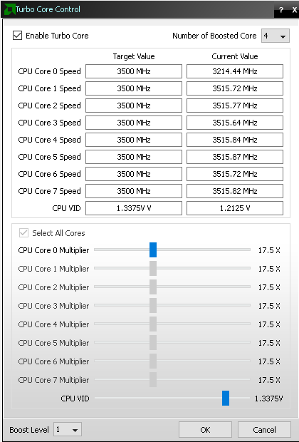
In the Turbo Core Control window on the top right side, you will see the drop-down menu which lets you select the number of cores you want to overclock, change it according to your preferences. On the top left side make sure "Enable Turbo Core" is checked. In this Window, you will see what the CPU core multiplier is by default.


 Now, increase the CPU 0 core multipler slowly by increments of 1 or 0.5. You want to make sure that your system is stable at that multiplier. If you set this value too high the system might restart and the default values will be restored. Not that along with setting the multiplier to 20X, I have also increased the voltage little bit as I saw it was giving a better performance at this value. Don't set the voltage too high as it may damage your system permanently. 


Locking page files in memory

Doing this increased the hash rate around 30%.
To enable the lock pages in memory option
  1. On the Start menu, click Run. In the Open box, type gpedit.msc.
  2. The Group Policy dialog box opens.
  3. On the Group Policy console, expand Computer Configuration, and then expand Windows Settings.
  4. Expand Security Settings, and then expand Local Policies.
  5. Select the User Rights Assignment folder.
  6. The policies will be displayed in the details pane.
  7. In the pane, double-click Lock pages in memory.
  8. In the Local Security Policy Setting dialog box, click Add user or group.
  9. In the window that opens, enter your computer's username and click on search names and it will add your user account. I would suggest adding both your account and the administrator account there.
  10. Click on Ok and then apply.

Performance after changing the setting to get max output

Minergate: Monero hash rate- 190-200H/s on CPU,  650-700H/s on GPU. Whenever I start mining( auto mining, which according to them mines currencies which give you the best profit that time) it only mines Monero with both CPU and GPU. I manually started Ethereum mining to see how much hash rate I am getting after all the optimization. Even after all the optimizations, I was only getting 13-13.5Mh/s.

Nicehash: Monero hash rate- 310-330H/s on CPU. Ethereum hash rate- 28.5Mh/s. So, as you can see from the results Nicehash was performing a lot better than Minergate.

Minergate vs Nicehash

As you can see from the results Nicehash is far better than Minergate. If you are using Linux setting up Nicehash may be a little difficult compared to Minergate. If you are mining on a system like this, it may be a month or so before you get your first payment. Nicehash pays you when your balance reaches 0.01BTC for external wallets. No matter which coin you are mining Nicehash automatically converts your earnings to Bitcoin and keeps it until it reaches 0.01BTC. 


Note: Please try all these modifications at your own risk.


Detecting Parallelogram in Images

Detecting Parallelogram in Images


The steps used in the detection of a parallelogram

  1. Load the raw image and convert it to grayscale using the formula
     2.   Plot the histogram to see what could be the threshold value for thresholding
     3.   Use canny edge detection to detect the edges
     4.   Threshold the image
     5.   Apply hough transform to get the accumulator and the points corresponding to
            each accumulator array value.
     6.  Find every Two pairs of parallel lines and then find two more pairs of parallel lines
            and find their intersection points.
     7.  Check if the intersection points are actually a part of the edge.
     8.  Using the intersection point found, draw the line on the original image to show the
            Parallelogram.


1.  Loading image and converting it to grayscale


Fig 1: The original color image(left) and the grayscale image(right)


In this part, we load the raw image and convert it into a grayscale image. The data format of the raw image is as follows:
The data arrangement for the interleaved raw image format is illustrated below, assuming an image of size  M X N (rows X columns).
R(0,0) G(0,0) B(0,0) R(0,1) G(0,1) B(0,1) ……………………………………R(0,N-1) G(0,N-1) B(0,N-1)
R(1,0) G(1,0) B(1,0) R(1,1) G(1,1) B(1,1) ……………………………………R(1,N-1) G(1,N-1) B(1,N-1)

When we load the raw image, it is thrice as wide as its grayscale image would be. To convert it to grayscale we loop over the raw image and multiply the R,G,B with their respective ration in luminance formula.
for i in range(0,rows):
    for j in range(0,columns):
        img_gray_man[i][j] = (0.3*img_color[i][j*3] +0.59*img_color[i][j*3+1] +0.11*img_color[i][j*3+2])


 2.  Plotting a histogram to get the threshold
       The histogram of an image can be used to get an idea of what the threshold value should be. The point where we see a deep valley between two peaks in the histogram can be a value of the threshold. Instead of a manual threshold, automatic thresholding can also be used to get the threshold value but during this project, I found that the automatic thresholding technique which uses peakiness to get the threshold value doesn’t perform well in all the cases. Peakiness depends on finding a valley between two peaks in the histogram of an image but if the histogram is a convex shape, i.e. it has a single peak the peakiness method doesn’t perform well.

Fig 2: Histogram of image 1.
In Fig 2 we see that the threshold value can be anything in the middle of these peaks.

 3.  canny edge detection to detect the edges
          In this part, we perform the Canny edge detection to detect the edges in the image. The Canny edge detection consists of 4 steps which are:
●     Use gaussian smoothing to smooth the image. In this step, we apply a Gaussian filter to the image to remove noise.
●     Apply the edge operator to the image. This will give back the image with thick edges.
●     Quantize the gradient angle of the edges into three sectors.
●     Apply non-maxima suppression to the image with thick edges to get thin edges. This is done with the help of the gradient angles found in the previous step. We take the gradient of a pixel location and see the value of the gradient along the sector of its gradient angle. If it is less than any of the two pixels along that direction we set its value to zero.

            The formula to calculate the gradient and the gradient angles are as follows:


Fig 3: Formula to calculate gradient value and gradient angle( Source: Wiki)


Fig 4: Value of Sectors depending on gradient angle


   g = create_guassian_mask([3,3] , 0.0 , 1)   
   img_after_gaussian_mask = (apply_map(image , g , False) / sum(sum(g)))  
   #sobels operator returns the gradient magnitude array and the gradient direction array  
   image_after_sobels_operator , theta = edge_operator(img_after_gaussian_mask , "sobels")  
   quantized_theta = quantize_gradient_angle_to_secotrs(theta)  
   image_after_non_maxima_suppression = non_maxima_suppression(image_after_sobels_operator , quantized_theta)  
   return image_after_non_maxima_suppression      
This function is in the edgedetction.py file and all the functions it calls are also in the same file. These files get called by the houghtransform.py file. All these files can be found on my Github. It first creates a gaussian mask ‘g’ which is then applied to the image to smooth it and remove noise. Then we use the Sobels edge operator to get the gradient magnitudes and gradient angles. These gradient angles are then quantized by the function quantize_gradient_angle_to_secotrs.


Fig 5: Image after canny edge detection


4.  Threshold Image
       In this part we threshold the image. We use the threshold value we found above to convert the grayscale image to binary image. This is based on simple comparison, if the value of the pixel is above threshold set it to 255 and if it is below set it to 0( this will be reversed depending on if you want the background to be black and foreground to be white or vice versa). After you threshold the image you will get a binary image on which we can perform the hough transform.


Fig 6: Image after thresholding

5.    Apply hough transform
       In this step we apply the hough transform to get the accumulator and the positions of the pixels that correspond to incrementing a particular location in the accumulator.

The Hough transform is a feature extraction technique used in image analysis, computer vision, and digital image processing.[1] The purpose of the technique is to find imperfect instances of objects within a certain class of shapes by a voting procedure. This voting procedure is carried out in a parameter space, from which object candidates are obtained as local maxima in a so-called accumulator space that is explicitly constructed by the algorithm for computing the Hough transform.
The simplest case of Hough transform is detecting straight lines. In general, the straight line y = mx + b can be represented as a point (b, m) in the parameter space. However, vertical lines pose a problem. They would give rise to unbounded values of the slope parameter m.


Fig 7: Formula for the line in theta, r

Fig 8


Hough Transform Algorithm (for straight lines)
  1. Quantize the parameter space appropriately
  2. Assume that each cell in the parameter space is an accumulator. Initialize all cells to zero
  3. For each point (x,y) in the image space increment by 1 each of the accumulators that satisfy the equation
  4. Maxima in the accumulator array correspond to the parameters of model instances


Hough transform implementation:
  1. First I create the theta array depending on the step size using the following code:
     def get_theta_list(step_size):
    if 360 % step_size != 0:
        print("step_size not a factor of 180")
    no_of_steps = int(round(360/step_size))

    return np.linspace(0 , 360 ,no_of_steps )+(round(step_size/2))

  1. Then for all the points in the binary image that are foreground( 0 or 1 depending on how the foreground is represented) we increment the value of the accumulator array for all the values of theta in theta array that we got in previous step. We also store the location of the points that incremented a particular position in accumulator array in the dictionary accumulator_positions The key of this dictionary is the p or r  and the theta and the value is the list of points. The code to create the accumulator array is:

def increment_accumulator(image , thetas , theta_step_size  = step_size_theta, p_step_size  = step_size_p):
    accumulator_positions = {}
    n,m = image.shape
    accumulator  = create_accumulator(len(thetas) , p_step_size)
    accumulator_rows , accumulator_columns = accumulator.shape
    # this line get the index of all the points that are non zero in the binary image
    y_idxs, x_idxs = np.nonzero(image)
    for z in range(len(y_idxs)):
        i = y_idxs[z]
        j = x_idxs[z]
        for theta in thetas:
            theta_position_in_accumulator = int(round((theta)/step_size_theta))-1
            result = int(round((calculatep(theta , j , i)+diag_len)/step_size_p))
            accumulator[result][theta_position_in_accumulator] += 1
            #check if the point is already at this loc in dictionary
            if((result,theta_position_in_accumulator) in accumulator_positions.keys()):
                accumulator_positions[result,theta_position_in_accumulator].append((i,j))
            else:
                accumulator_positions[result,theta_position_in_accumulator] = [(i,j)]

    return accumulator , accumulator_positions


  1. Once we get the accumulator array we threshold it to remove all the points that may not correspond to a straight line.
  2. After thresholding we find the points of intersection of parallel lines to get the corners of the parallelogram. To do this first we find two pair of parallel lines from the accumulator_pos dictionary and check if these parallel lines are some distance apart to prevent detecting very narrow parallelograms which may be of the same edge. Then we find two more parallel lines using the same dictionary and check if they are some distance apart. Now we have 4 lines which may form a parallelogram.
  3. To check if the 4 lines actually form a parallelogram we use the equation of these four lines and find the four intersection points. Then we check if there are enough points in between these corner points to say if they actually for a parallelogram. To check this we can find the distance between the corner points and then check if the ratio of the distance and the number points between these corner point is above some threshold.
  4. Once we have the corner points of the parallelogram we can draw it over the original image using the cv2.line function.


Fig 6: Image if the accumulator array(X-axis: theta , Y-axis:p)


Fig 7: Image after thresholding of accumulator array


Image after drawing the parallelogram over it

Saturday, 27 January 2018

Region Segmentation in Image

Region Segmentation

What we will be doing on this blog?
We will segment an image into two regions ie foreground and background and then assign a unique label to each object in the foreground.

A region is a subset of an image. Region segmentation is grouping the pixels in an image into regions. 

To segment an image into different regions we need to differentiate the regions. There can be many things on which the differentiation can be done. In this blog, we will use the pixel intensity as differentiating factor. For example, let's assume we have an 8-bit(pixel values can be from 0 to 255) grayscale image and we decide that every pixel above the intensity 50 belongs to the foreground and less than equal to 50 belongs to the background. In this way, we have created 2 different regions in the image ie the foreground and the background. This method of deciding the foreground and the background based on a threshold value is called thresholding.


Thresholding
There are three types of thresholding:
  1. Automatic Thresholding
  2. P-tile Thresholding (Manual thresholding)
  3. Choose a threshold value by looking at the image
P-tile Thresholding(Manual): If we know that one or more objects occupy a fixed area on the image, then we can choose a threshold T such that p percent of pixels would have gray level value < T.

Automatic Thresholding: In this method, the program automatically chooses one or more threshold values and segment the image based on those values.

For simplicity, in this post, we will be setting the threshold manually by looking at the image. Looking at the image directly may not give you an idea of what the threshold should be so what we can do is plot the histogram of the image and try to find the threshold from that. For example look at the image(image 1) below, you may not be able to see what the threshold should be. 


Now see the histogram of this image. In the histogram, you can see that there are two peaks, one with a peak around 70 and the other with a peak around 180. These two peaks represent the two regions in the image. The background is dark so the peak corresponding to the background will be the one peak around 70 and the coins are light gray so the peak corresponding to it is around 180.
So, to pick a threshold we select a low value between these peaks. In this histogram, this value will be around 110.

Histogram: x-axis is the pixel intensity and the y-axis is the number of pixels at that intensity.


Segmenting the image into foreground and background


Now that we have got the threshold value next step is to convert the image into a binary image. A binary image is an image with only 2 pixel-intensities ie 0 and 1. Let us represent the background by 0 and the foreground by 1(this is not compulsory you can use the opposite of it as well). To convert the grayscale image to binary image, create a new zero array of the size of the original image, loop through all the pixels of the original image. If the intensity of the pixel is above the threshold set the corresponding pixel in the zero array to 1 and let it be zero otherwise. Look at the code below to understand better.

 rows,columns = image.shape  
 binary_image = np.zeros((rows , columns))  
   
 for i in range(0, image_rows_len):  
   for j in range(0, image_columns_len):  
     if(image[i][j] > 110):  
       binary_image[i][j] = 1  


After converting the image to binary image you would get something like this:


Now that we have the image of two regions we can see that it has 10 components(10 coins). We can assign a unique label to each of these components using the component labeling algorithm. Before I tell you what this algorithm is there are a few terminologies that you should know.

The first one is Neighbors.


The following image shows the result of the labeling algorithm. 


The connected component labeling algorithm is the following:
This algorithm uses the 4 neighbor definition of connected component ie two pixels share a boundary and both of them belong to the foreground then they are considered as connected. In other words, two pixels are connected if there a 4-path between them.


 1
 2
 3
 4
 5
 6
 7
 8
 9
10
11
12
13
14
15
16
17
18
19
20
21
22
23
24
25
26
27
28
29
30
31
32
33
34
35
36
37
38
39
40
41
42
43
44
45
46
47
48
49
50
51
52
53
54
55
56
57
58
59
60
61
62
63
64
65
66
67
68
69
70
71
72
73
74
75
76
77
78
79
80
81
82
83
84
85
86
87
def segment_region(img):
    labels = img * 0
    n, m = img.shape
   
    eqivalenceList = []
    # increment label number only if you assign a new label
    label = 1
    
    #looping through every pixel of the binary image
    for i in range(0, n):
        for j in range(0, m):
            #we only run this algorithm on foreground pixels
            if (img[i][j] == 1):
                # check if row above exists
                if (i > 0 and j > 0):
                    # we are not in the top row or leftmost column, label pixel if 1
                    if (img[i][j] == 1):
                        # check if the pixel above it has a label
                        if (labels[i - 1][j] != 0):
                            labels[i][j] = labels[i - 1][j]
                        else:
                            # pixel above doesn't have a label, check left neighbor pixel
                            if (labels[i][j - 1] != 0):
                                labels[i][j] = labels[i][j - 1]
                            else:
                                # it doesn't have a top or left neighboring labelled pixel so assign a new pixel
                                labels[i][j] = label
                                label += 1
                        # if both top or left neighboring pixels are there, we have to insert
                        # them in equivalence table
                        #this is the case when we are assigning label to current pixel and its top and left neighbor have different labels
                        #As all three of them would be connected in a 4 path they all should belong to same label(region)
                        if(labels[i - 1][j] != 0 and labels[i][j - 1] != 0 and labels[i][j - 1] != labels[i - 1][j]):
                            # check if this pair of values are not already in the list
                            inserted = False
                            for evalList in eqivalenceList:
                                if (labels[i - 1][j] in evalList):
                                    evalList.append(labels[i][j - 1])
                                    inserted = True
                                    break
                                elif (labels[i][j - 1] in evalList):
                                    evalList.append(labels[i - 1][j])
                                    inserted = True
                                    break
                            if (not inserted):
                                eqivalenceList.append([labels[i][j - 1], labels[i - 1][j]])

                else:
                    # we are in the top row or the leftmost column
                    
                    # check if we are in the top row. If we are in the top row and there is a pixel on the left
                    # that is labelled , then we can just copy the label.
                    if (i == 0 and j > 0):
                        if (labels[i][j - 1] != 0):
                            labels[i][j] = labels[i][j - 1]
                    # we are in the leftmost column 
                    # check if we are in the leftmost column. If we are in the leftmost column and there is a pixel on the top
                    # that is labelled , then we can just copy the label.
                    if (i > 0 and j == 0):
                        if (labels[i - 1][j] != 0):
                            labels[i][j] = labels[i - 1][j]
                    # case 0,0, top most row , leftmost column
                    if (i == 0 and j == 0):
                        if (img[i][j] == 1):
                            labels[i][j] = label
                            label = label + 1

    # length of equivalence list does not tell the number of regions. foreground that are one pixel in area
    # or other regions in which only one label is set to all the pixels in the regions will not be in the
    # equivalance list

    #Right now each region may contain more than one labels. Here we set the minimum label that the region has to that region.
    for evalList in eqivalenceList:
        for i in range(0, n):
            for j in range(0, m):
                if (labels[i][j] in evalList):
                    labels[i][j] = min(evalList)

    # to get the total number of regions see the number of different values in labels array
    # background will be given label 0
    diffLabels = []
    for i in range(0, n):
        for j in range(0, m):
            if (labels[i][j] not in diffLabels):
                diffLabels.append(labels[i][j])

    return diffLabels, labels